
Replications for introduction to g-methods: standard linear regression (part 0)
Published:
This tutorial series aim to replicate g-methods explained in this paper by Naimi, A. I., Cole, S. R., and Kennedy, E. H (2017)1 using R. Originally, the paper used SAS to demonstrate g-methods.
In this tutoiral, we will focus on replicating the data generation and estimates from the standard linear regression model to understand the crude differences between treated and control groups.
The empirical setting is to treat HIV with a therapy regimen (\(A\)) in two time periods (\(t = 0, t = 1\)). Additionally, we measure the time-varying confounder, HIV viral load (\(Z\)) at times \(t = 0\) and \(t = 1\). Note that this time-varying confounder is measured prior to the treatment administered at each time period. Also, we assume \(Z\) at time 0 is 1 (high, bad health condition) for all subjects. Our outcome is the CD4 count (cells/mm\(^3\)) observed at \(t = 2\).
Thus, we have:
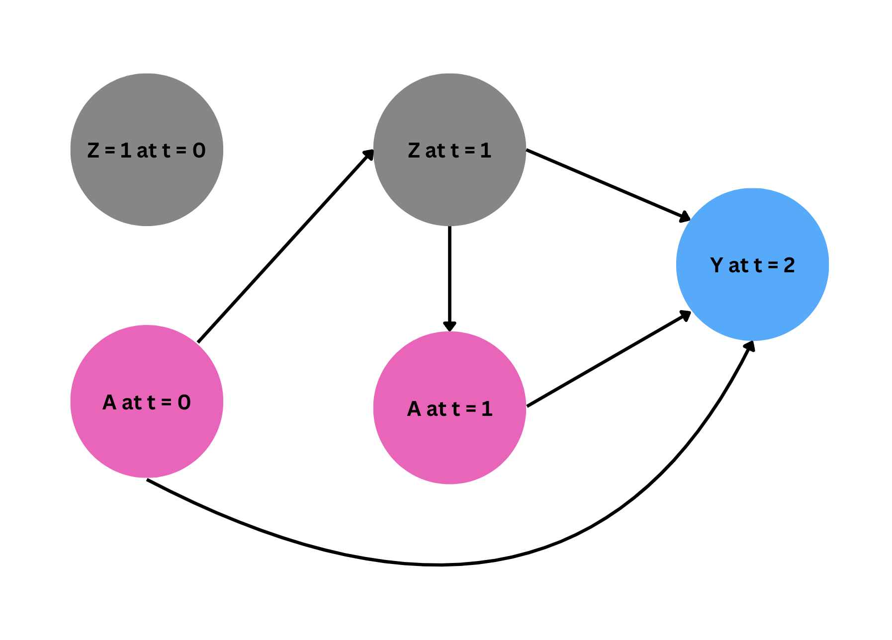
Under the identifying assumptions described in the paper, we will estimate the average casual effect of always taking treatment (\(a_0 = 1, a_1 = 1\)), compared to never taking treatment (\(a_0 = 0, a_1 = 0\)) in both time periods. For notation, we are using subscripts to indicate time periods.
# Read packages
library(tidyverse)
library(ascii)
We will begin with the standard linear regression to peak the crude differences between always-treated and never-treated in their outcome.
# Replication

# Data in Table 1
# A0: Treatment at time 0 (for HIV)
# Z1: HIV viral load measurement prior to time 1 (Higher: Worse health condition)
# A1: Treatment at time 1
# Y: Mean of CD4 counts
# N: Number of subjects


a0 <- c(0, 0, 0, 0, 1, 1, 1, 1)
z1 <- c(0, 0, 1, 1, 0, 0, 1, 1)
a1 <- c(0, 1, 0, 1, 0, 1, 0, 1)
y <- c(87.288, 112.107, 119.654, 144.842, 105.282, 130.184, 137.720, 162.832)
n <- c(209271, 93779, 60657, 136293, 134781, 60789, 93903, 210527)

data <- data.frame(a0, z1, a1, y, n)
Replicates for Table 1
| a0 | z1 | a1 | y | n |
|---|---|---|---|---|
| 0 | 0 | 0 | 87.288 | 209271 |
| 0 | 0 | 1 | 112.107 | 93779 |
| 0 | 1 | 0 | 119.654 | 60657 |
| 0 | 1 | 1 | 144.842 | 136293 |
| 1 | 0 | 0 | 105.282 | 134781 |
| 1 | 0 | 1 | 130.184 | 60789 |
| 1 | 1 | 0 | 137.720 | 93903 |
| 1 | 1 | 1 | 162.832 | 210527 |
Now, we fit the data with standard linear regression models to replicate Table 2.
Standard Linear Regressions
# Section 1
# Standard linear regression models in Table 2
# Not considering standard error estimation

# Crude model
lm_1 <- lm(y ~ a0 + a1 + a0*a1, data = data, weights = n)

# Z-Adjusted model
lm_2 <- lm(y ~ a0 + a1 + a0*a1 + z1, data = data, weights = n)

# A0 only model
lm_3 <- lm(y ~ a0, data = data, weights = n)

# Z1-Adjusted A0 Only Model
lm_4 <- lm(y ~ a0 + z1, data = data, weights = n)

# A1 Only Model
lm_5 <- lm(y ~ a1, data = data, weights = n)

# Z1-Adjusted A1 Only Model
lm_6 <- lm(y ~ a1 + z1, data = data, weights = n)
We now check the crude difference in mean CD4 count for the always treated compared to the never treated. In the first model, \(\hat{\beta} = 60.96\) as reported in the paper. In model two, \(\hat{\beta} = 43.01\), which is slightly larger than as it is reported. This estimate is the \(Z_1\)-adjusted difference in mean CD4 count for the same contrast. The results from other four models are reported in Table below.
In the next post, we will move onto fitting g-methods to the data in Table 1, beginning with g-formula.
table2 <- data.frame(model = c("m1", "m2", "m3", "m4", "m5", "m6"),
                     beta1 = c(lm_1$coefficients["a0"] + lm_1$coefficients["a1"] + lm_1$coefficients["a0:a1"],
                               lm_2$coefficients["a0"] + lm_2$coefficients["a1"] + lm_2$coefficients["a0:a1"],
                               lm_3$coefficients["a0"],
                               lm_4$coefficients["a0"],
                               lm_5$coefficients["a1"],
                               lm_6$coefficients["a1"])) %>%
  mutate(beta1 = round(beta1, 2))
Replicates for Table 2
| model | beta1 |
|---|---|
| m1 | 60.96 |
| m2 | 43.01 |
| m3 | 27.08 |
| m4 | 18.03 |
| m5 | 38.91 |
| m6 | 25.01 |
Naimi, A. I., Cole, S. R., & Kennedy, E. H. (2017). An introduction to g methods. International journal of epidemiology, 46(2), 756-762. ↩