
Replications for introduction to g-methods: g-formula (part 1)
Published:
This tutorial series aims to replicate g-methods explained in this paper by Naimi, A. I., Cole, S. R., and Kennedy, E. H (2017)1 using R. Originally, the paper used SAS to demonstrate g-methods.
In this tutorial, we will focus on replicating the results using g-formula to estimate the average causal effects of always taking treatment compared to never taking treatment. From our knowledge of the data-generating process, we know this average causal effect to be \(50\). In our tutorial, we will pay more attention to computation rather than proofs to perform replications.
Reminder: Our Settings
 Under the identifying assumptions described in the paper, we will estimate the average causal effect of always taking treatment ($a_0 = 1, a_1 = 1$), compared to never taking treatment ($a_0 = 0, a_1 = 0$) in both time periods. For notation, we are using subscripts to indicate time periods.
G-formula with computation
The g-formula can be used to estimate the average potential outcome level that would be observed in the population (that is, marginal outcome2) under a hypothetical treatment intervention. We estimate the marginal mean of Y that would be observed if \(A_0\) \(A_1\) were set to some values \(a_0\) and \(a_1\) hypothetically using the estimator on the right-hand side of the question below.
\[\begin{align*} E(Y^{a_0, a_1}) = \textstyle\sum_{a_1, z_1, a_0} \,\,&E(Y | A_1 = a_1, Z_1 = z_1, A_0 = a_0)\\\ &P(A_1 = a_1 | Z_1 = z_1, A_0 = a_0)\\\ &P(Z_1 = z_1 | A_0 = a_0)\\\ &P(A_0 = a_0) \end{align*}\]Because we hypothetically intervene in treatment, we can simplify our estimator. This simplification is possible because, as we intervene in treatment, the probability density for treatment becomes irrelevant; it is already determined at the point of our intervention.
\[\begin{align*} E(Y^{a_0, a_1}) = \textstyle\sum_{z_1} \,\,&E(Y | A_1 = a_1, Z_1 = z_1, A_0 = a_0)\\\ &P(Z_1 = z_1 | A_0 = a_0) \end{align*}\]Note that the right side of the equation is essentially equivalent to computing a weighted average of \(Y\) marginalized over \(Z_1\) given \(A_0\).
In our scenario, we compute two expected values to estimate our estimand: the average causal effects of always being treated compared to never being treated. Thus, we are interested in computing two expected values for the always-treated intervention \(E[Y^{a_0 = 1, a_1 = 1}]\), and for the never-treated intervention, \(E[Y^{a_0 = 0, a_1 = 0}]\). Finally, our estimand of interest (\(\hat{\tau}\)) is calculated as:
\[\hat{\tau} = E[Y^{a_0 = 1, a_1 = 1}] - E[Y^{a_0 = 0, a_1 = 0}]\]R-codes below demonstrate how we compute these expected values step-by-step.
# Replication

# Data in Table 1
# A0: Treatment at time 0 (for HIV)
# Z1: HIV viral load measurement prior to time 1 (Higher: Worse health condition)
# A1: Treatment at time 1
# Y: Mean of CD4 counts
# N: Number of subjects


a0 <- c(0, 0, 0, 0, 1, 1, 1, 1)
z1 <- c(0, 0, 1, 1, 0, 0, 1, 1)
a1 <- c(0, 1, 0, 1, 0, 1, 0, 1)
y <- c(87.288, 112.107, 119.654, 144.842, 105.282, 130.184, 137.720, 162.832)
n <- c(209271, 93779, 60657, 136293, 134781, 60789, 93903, 210527)

data <- data.frame(a0, z1, a1, y, n)
Always treated intervention
# E[Y^{1, 1}]

# The total number of subjects in the A0 = 1 stratum
a0_1_n <- data %>%
  filter(a0 == 1) %>%
  summarise(a0_1_n = sum(n)) %>%
  pull()

#  Weights for Z1 = 0 and Z1 = 1 among those with A0 = 1
weight <- data %>%
  filter(a0 == 1) %>%
  group_by(z1) %>%
  summarise(weight = sum(n) / a0_1_n) %>%
  select(z1, weight)

# Compute expectation’s value for always treated
expected_value_always_treated <- data %>%
  filter(a0 == 1 & a1 == 1) %>%
  left_join(weight, by = "z1") %>%
  mutate(weighted_y = y * weight) %>%
  group_by(a0, a1) %>%
  summarise(weighted_sum = sum(weighted_y))

expected_value_always_treated
Never treated intervention
# E[Y^{0, 0}]
# Never treated

# The total number of subjects in the A0 = 0 stratum
a0_0_n <- data %>%
  filter(a0 == 0) %>%
  summarise(a0_0_n = sum(n)) %>%
  pull()

# Weights for Z1 = 0 and Z1 = 1 among those with A0 = 0
weight <- data %>%
  filter(a0 == 0) %>%
  group_by(z1) %>%
  summarise(weight = sum(n) / a0_0_n) %>%
  select(z1, weight)

# Compute expectation’s value for those never treated
expected_value_never_treated <- data %>%
  filter(a0 == 0 & a1 == 0) %>%
  left_join(weight, by = "z1") %>%
  mutate(weighted_y = y * weight) %>%
  group_by(a0, a1) %>%
  summarise(weighted_sum = sum(weighted_y))

expected_value_never_treated
Finally, we report the results in Table below. We find that the average causal effect (\(\hat{\tau}\)) is \(50 = 150-500\) as shown by the authors.
| a0 | a1 | weighted_sum |
|---|---|---|
| 1 | 1 | 150.0621 |
| 0 | 0 | 100.0370 |
This approach to computing the value of the g-formula is called nonparametric maximum likelihood estimation.
G-formula with parametric models
However, we often use simulation from parametric regression models to construct a g-formula estimator. This approach is typically the most realistic when dealing with many covariates in our data. Now, we will discuss how to use parametric regression models to apply the g-formula. Although the web supplement includes the procedures, the results from the parametric g-formula are not included in the main article.
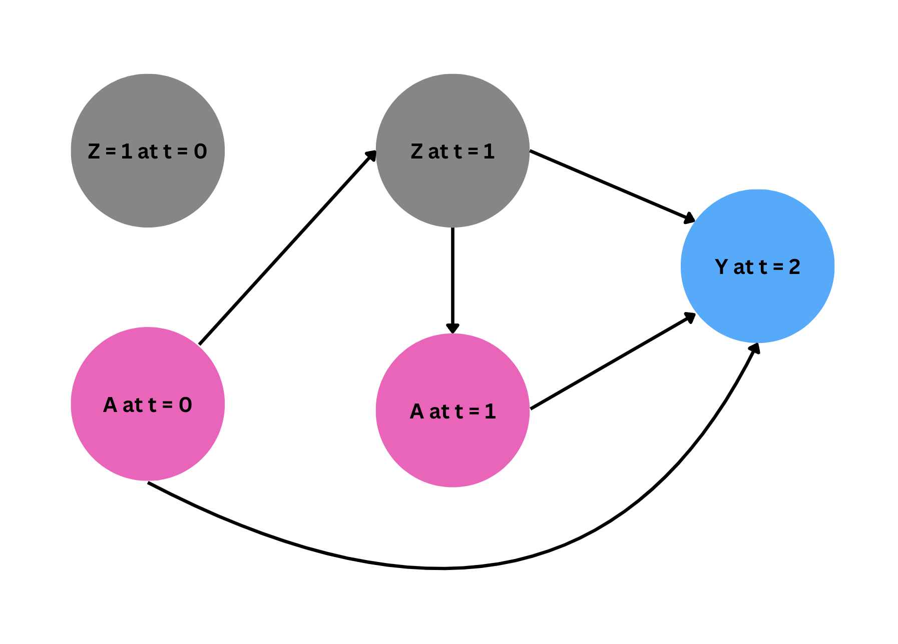
As the first step, we fit a model for each compoment of the likelihood in our estimator following the order of the events in time. As the below digram shows, \(Z_1\) is affected by \(A_0\), and $A_1$ is administered depending on the level of $Z_1$. Finally, $Y$ is affected by all treatments \(A_0, A_1\) and time varying confounder $Z_1$ (recall $Z_0$ is fixed at 1 for all observations, and thus gives us no additional information).
Given this relationship of the variables, we fit the models in R.
Step 1: Fit models
# Step 1: Fit a model for each component of the likelihood
# Note we disregard the number of subjects for each stratum and weigh them equally

z1_model  <- glm(z1 ~ a0, family = binomial())
a1_model <- glm(a1 ~ z1, family = binomial())
y_model <- lm(y ~ a1 + z1 + a0 + a1*a0, data = data)
Note that we use logistic models for $Z_1$ and $A_1$ since they are binary variables and a linear model for $Y$. All these models include parametric assumptions about the relationships between the variables, which may bias our estimates if these assumptions do not hold in our data-generating processes.
Step 2: Generate simulated values for $A$, $Z$ and $Y$ using models
Using our models, we now generate simulated values for each variable $A$, $Z$, and $Y$. For the baseline variable $A_0$, we randomly sample it with replacement from the data, with $n = 1,000,000$. Then, we feed these simulated values into the subsequent models that consider the sequence of events. Specifically, to simulate $Z_1$, we use the $Z_1$-model to predict the probabilities of having $Z_1 = 1$ given the simulated values of $A_0$ from the previous step and use \texttt{rbinom} to generate simulated binary values for $Z_1$. Next, we feed these simulated values $(A_0, Z_1)$ into the $A_1$-model to generate binary simulated values for $A_1$, following a similar procedure. Finally, using the simulated values of $A_0, Z_1$ and $A_1$, we simulate $Y$ using the $Y$-model.
# Step 2: Generate simulated values
set.seed(78419)

sim_n = 1000000

a0_sim <- data.frame(a0 = sample(a0, size = sim_n, replace = TRUE))


# simulation for z1 using the z1 model that is fitted with original data
# n = number of simulation
# prob = predicted probability from the z1 model

z1_sim <- rbinom(n = sim_n,
                 size = 1,
                 prob = predict(z1_model,
                                newdata = a0_sim,
                                type = "response"))

# simulation for a1 using the a1 model that is fitted with original data
# n = number of simulation
# prob = predicted probability from the a1 model

a1_sim <- rbinom(n = sim_n,
                 size = 1,
                 prob = predict(a1_model,
                                newdata = data.frame(z1 = z1_sim),
                                type = "response"))

# simulation for y using the y model that is fitted with original data
# n = number of simulation
# prob = predicted probability from the y model

y_sim <- predict(y_model,
                   newdata = data.frame(a0 = a0_sim,
                                        z1 = z1_sim,
                                        a1 = a1_sim),
                   type = "response")
Step 3: Intervene on treatment to compute g-formula using simulation
To estimate the average causal effects of always being treated compared to never being treated, we now hypothetically intervene on treatment according to each scenario using the simulated data. Then, we compute the differences in means for each scenario (always treated—never treated).
# Step 3: Intervene on treatment to compute g-formula using simulation
data_sim <- data.frame(a0 = a0_sim,
                       z1 = z1_sim,
                       a1 = a1_sim,
                       y = y_sim)

# always treated
always_treated <- predict(y_model,
                   newdata = data_sim %>%
                     mutate(a0 = 1,
                            a1 = 1),
                   type = "response")

# never treated
never_treated <- predict(y_model,
                         newdata = data_sim %>%
                           mutate(a0 = 0,
                                  a1 = 0),
                   type = "response")

# Compute the average potential outcome under each intervention scenario
potential_y <- data.frame(
  a0 = c(1, 0),
  a1 = c(1, 0),
  potential_outcome = c(mean(always_treated), mean(never_treated)))
We now report the results from the parametric g-formula below. As we see, $\hat{\tau}_{\text{parametric}}$ is equal to $43.037 = 146.4731 - 103.4361$. This estimate is lower than the true causal effect we already know from the data generation process, indicating our parametric models may be misspecified, leading to biased estimates.
| a0 | a1 | potential_outcome |
|---|---|---|
| 1 | 1 | 146.4731 |
| 0 | 0 | 103.4361 |
Using the parametric models, however, we can more easily estimate potential outcomes under other intervention scenarios, as shown below.
# other intervention scenarios

# natural course
natural_course <- predict(y_model,
                   newdata = data_sim,
                   type = "response")

# treated only at time 0
treated_time0 <- predict(y_model,
                   newdata = data_sim %>%
                     mutate(a0 = 1,
                            a1 = 0),
                   type = "response")

# treated only at time 1
treated_time1 <- predict(y_model,
                   newdata = data_sim %>%
                     mutate(a0 = 0,
                            a1 = 1),
                   type = "response")

potential_y <- data.frame(
  a0 = c(1, 0, "natural course"),
  a1 = c(0, 1, "natural course"),
  potential_outcome = c(mean(treated_time0), mean(treated_time1), mean(natural_course)))
The results from other interventions are reported below.
| a0 | a1 | potential_outcome |
|---|---|---|
| 1 | 0 | 121.4661 |
| 0 | 1 | 128.4396 |
| natural course | natural course | 124.9453 |
Parametric models used in this paper, such as generalized linear models, assume a linear relationship between the covariates ($A, Z$) and the response variable ($Y$). This linearity is modeled either directly through the parameters or indirectly through a transformation facilitated by a link function. While effective under certain conditions, these models are limited by their assumption of linearity and may lead to biased estimates if any of these models are misspecified, as illustrated in our example. Machine learning modeling, which can accommodate more complex, non-linear relationships, offers a flexible alternative to traditional parametric modeling
Switch to Marginal Structural Models (MSM)
To further enhance our analysis, we turn to marginal structural models (MSM). These models map the marginal summary (e.g., average) of potential outcomes to the treatment trajectories and parameters of interest, $\tau$. Thus, they require far less modeling for time-varying variables than approaches like the g-formula, which necessitates modeling for $P(Z_1 = z_1 | A_0 = a_0)$, in our example. The next tutorial will cover steps to fit marginal structural models for our causal question (always treated vs. never treated).
Naimi, A. I., Cole, S. R., & Kennedy, E. H. (2017). An introduction to g methods. International journal of epidemiology, 46(2), 756-762. ↩
My two cents: the term marginal in plain English usually means of less importance. But in our context, the term marginal is used to indicate population level outcome in contrast to individual level outcome. In some sense, it might make sense because it would be best if we are able to estimate individual treatment effects. As it is often not very feasible, we instead rely on population level estimates, which could be less important in some sense. However, considering that the population encompasses all individuals, it can sometimes be puzzling why we refer to it as marginal, as it is certainly bigger! ↩