Replications for introduction to g-methods: marginal structural models (part 2)

This tutorial series aims to replicate g-methods explained in this paper by Naimi, A. I., Cole, S. R., and Kennedy, E. H (2017)¹ using R. Originally, the paper used SAS to demonstrate g-methods.

In this tutorial, we will focus on replicating the results using marginal structural models to estimate the average causal effects of always taking treatment and compared to never-taking treatment. From our knowledge of the data-generating process, we know this average causal effect to be \(50\). In our tutorial, we will pay more attention to computation rather than proofs to perform replciations.

Reminder: Our Settings

The empirical setting is to treat HIV with a therapy regimen ($A$) in two time periods ($t = 0, t = 1$). Additionally, we measure the time-varying confounder, HIV viral load ($Z$), at times $t = 0$ and $t = 1$. Note that this time-varying confounder is measured before the treatment is administered at each time period. Also, we assume $Z$ at time 0 is 1 (high, bad health condition) for all subjects. Our outcome is the CD4 count (cells/mm$^3$) observed at $t = 2$. 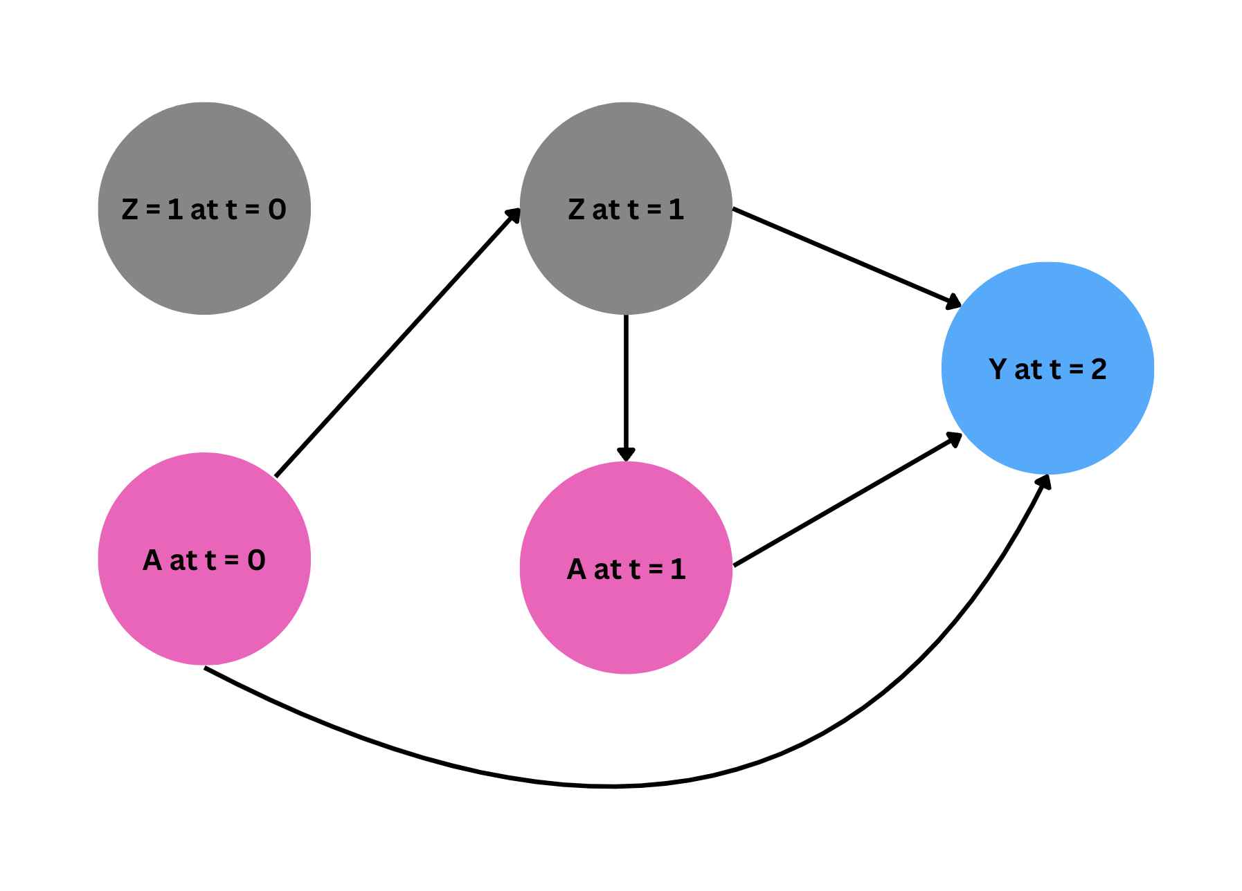Thus, we have: Under the identifying assumptions described in the paper, we will estimate the average causal effect of always taking treatment ($a_0 = 1, a_1 = 1$), compared to never taking treatment ($a_0 = 0, a_1 = 0$) in both time periods. For notation, we are using subscripts to indicate time periods.

Marginal Structural Models

Marginal structural models typically relate a marginal summary (e.g., average) of potential outcomes to the treatment and parameter of interest ($\beta$). Inverse probability weighting is most commonly used to estimate the parameters of these models. Specifically, to estimate $\beta$, we calculate the predicted probabilities of the observed treatments at each time $t$, given prior covariates and treatments. By weighting the observed data by the inverse of these probabilities, we generate a ``pseudo-population’’ in which treatment at each time $t$ is no longer related to, and thus no longer confounded by, prior covariates and treatments. Consequently, weighting a parametric model for the outcome by the inverse probability of treatment allows us to account for the fact that both the time-varying covariates and the treatment affect subsequent treatment statuses.